Introduction

In the upcoming network upgrade, Ethereum is slated to roll out EIP-4844 (nicknamed proto-danksharding) to drastically reduce the costs of rollups when it comes to committing data on Ethereum. The main ingredient of this EIP is what’s known as a blob, which introduces the aptly named concept of blobspace, which aims to be counterpart to the concept of blockspace that we know today.

This article aims to approach the concept of blobspace, from the ground up. We will go through a quick overview of the problem of scaling a blockchain and how the concept of blobspace is the answer that Ethereum is betting on. Then we will delve into the more technical aspects of blobspace, first from the perspective of EIP-4844, since it’s about to roll out, and then we’ll quickly look into what “full danksharding” will entail in the future.

History

The problem: how to scale?

Given that you’re reading an article about blobspace, I take it you’re at least somewhat familiar with the blockchain trilemma that has to do with decentralization, security and scalability (If you’re not, you have some catching up to do!), so I’m pretty sure you get the drill. So, for the sake of brevity, I’m gonna grossly oversimplify the problem with these two statements that are gonna be relevant through the rest of this article:

1. We want everyone to be able to verify the blockchain by themselves, by running their own node on their own hardware.¹
2. A node must download every single block and run every single transaction in order to verify that the result is valid and consistent with the rest of the network.

These two statements together explain the scarcity of blockspace present today: Transaction fees are lower if there is more blockspace, but more blockspace means nodes have to do more work (bandwidth, computation, storage), which may end up going against the goal from Statement #1. So instead, we have a relatively small supply of blockspace – about 15 million gas per block — being met with a fairly high demand, which results in Ethereum’s infamous high gas fees.

The goal is to somehow make the two statements not contradictory: we want more blockspace, but without increasing the burden on the nodes that constitute the network.

The solution: sharding

A solution that had been taken for granted as being the future of Ethereum was sharding: the switch to Proof of Stake came the possibility of shuffling validators randomly across distinct shards of the blockchain, each shard being essentially its own mini-blockchain running in parallel to the Beacon Chain. That’s actually where the name “Beacon Chain” comes from, it was meant to be the beacon of randomness that would redirect validators to random shards. So even if each shard had on paper significantly less economic security, someone hoping to 51% attack a specific shard would still have to control 51% of the entire validator set, otherwise their chances of having their validators randomly assigned to the same shard are near zero.

While this all sounds good on paper, there were many problems to solve to actually get secure specifications for sharding, as well as a lot of questions to answer when it comes to cross-shard communication, backwards compatibility with existing contracts, etc. And while all the research, discussions, debates were ongoing, another scaling solution showed up and kind of changed the game: rollups.

The other solution: rollups

Without going into too much detail, you can think of a rollup as being its own blockchain that runs “on top” of Ethereum (hence the term Layer 2 or L2). Just like a blockchain, a rollup holds an internal state, executes transactions to compute state transitions, etc. We then introduce a new class of actors call sequencers which are in charge of batching (or *rolling up”) many Layer 2 transactions into a single Layer 1 transaction.

The gain in scalability comes with the fact that Ethereum’s validators and nodes aren’t burdened with the task of computing every single rollup transaction, but they still secure them and enforcing their validity. How is this possible? By having a smart contract on Ethereum that enforces some key constraints on what a rollup sequencer can do and take care of bridging assets.

Let’s see how this works for optimistic and zero-knowledge rollups:

• Optimistic Rollups: The L1 contract accepts all batches as valid, but enforces a delay before assets can be withdrawn out of the rollup
  • During this delay, anyone can submit a fraud proof if the sequencer acted malicious and committed an invalid transaction
• zkRollups: The L1 contract accepts all batches that come with a cryptographic validity proof
  • This validity proof is very short, typically logarithmic in size: squaring the number of L2 transactions only doubles the size of the proof!

In both cases, the L1 contract also allows users to manually push L2 transactions (e.g., to exit funds) in case the sequencer tries to censor users. The tagline for rollups is that they “inherit security from Ethereum”, since in order to reorg rollup blocks, you’d need to reorg Ethereum too, which is extremely hard and expensive to pull off.

There are plenty of design decisions and trade-offs when it comes to how the sequencers operate in practice, but that’s the general idea. For the rest of this article, what’s important to notice is that very little execution happens at Layer 1, what rollups need first and foremost is data. While Ethereum nodes don’t need to compute every single L2 transaction, they still need to have all data relevant to L2 transactions, otherwise bad things can happen:

• For optimistic rollups, a malicious sequencer could commit an invalid transaction that steals all funds, then withhold the data necessary for a fraud proof, then it’s a matter of waiting out the delay before the L1 contract lets them bridge out their ill-gotten funds.
• For zkRollups, a malicious sequencer can’t steal funds, but withholding data still allows them to censor and hold everyone’s funds hostage.

Since we want rollups to be trustless and censorship resistant like Ethereum, it’s crucial that all the data necessary to sync the rollup’s internal state is forcibly made available on Layer 1, since it’s by having the state that you can submit fraud proofs and withdraw funds from rollups.

The rollup-centric roadmap

The year is 2020, there is still plenty of work to be done on the transition to Proof-of-Stake, and there are no clear specifications for sharding. Various rollups are announcing testnet launches. Doing the math indicates that rollups will be able to scale to significantly more transactions per second than Ethereum will ever achieve with sharding alone.

As Vitalik puts it in his ethereum-magician post:

It seems very plausible to me that when [full execution sharding] finally comes, essentially no one will care about it. Everyone will have already adapted to a rollup-centric world whether we like it or not, and by that point it will be easier to continue down that path than to try to bring everyone back to the base chain for no clear benefit and a 20-100x reduction in scalability.

Basically, we could do the complex thing and scale Layer 1 execution, but all that would achieve is that rollup sequencers would say “oh cool, more data” and barely touch the execution that we took so long to shard. So instead, the plan is now to scale back the scope of sharding to merely data sharding – the execution will only happen on the Beacon Chain for the purposes of rollups (fraud proofs and validity proofs) and then validators assigned to random shards will only be in charge of serving rollup’s data to whoever asks for it.

With rollups in mind, the plan now becomes that Layer 1 will scale data (which is easier to do) and Layer 2 will convert this scalable data into scalable execution. If this sounds like Ethereum core devs giving up, that’s because it kind of is. But it’s a pragmatic decision! Unlike Ethereum, rollups can afford to move fast, and competing against each other drives innovation. This modular design keeps core protocol changes at a minimum, while the dream of safely scaling blockchains without sacrifices lives on.

Another underrated aspect of this rollup-centric roadmap is that rollups are much freer to innovate independently from each other: with the original sharding plans, every shard had the same EVM, same finality properties, same everything with the same exact tradeoffs². Betting on rollups means getting much more innovation at a much faster pace.

Danksharding

In another move of drastically simplifying things, Ethereum researcher Dankrad Feist proposed a different design in a document he titled New sharding design with tight beacon and shard block integration. With this design, we get rid of the concept of a shard being a mini-blockchain altogether. Instead, all we have are blobs that are constructed in a clever way (as we’ll see later) so that although blocks are filled with big blobs, each individual node only needs to do a very small amount of work to check that all the data is available.

Checking that all the data is available is what’s known in the business as a “data availability check” – without having to download all the data, your node can be convinced that all the data is there, if you ever need it. This solves the problem of rollup sequencers potentially withholding data: just like nodes won’t follow a fork that contains invalid transactions, nodes won’t follow a fork where data isn’t available – even if 99% of validators are maliciously trying to withhold data!

The main trade off that comes with danksharding is that constructing a block becomes a very heavy process in terms of bandwidth and computation, which is a centralizing force on block builders. Fortunately (but also, unfortunately), centralization of block builders is already happening due to MEV – builders already have beefy machines running the most optimized algorithms possible to squeeze value out of Ethereum’s blockspace. With danksharding, they will have the extra role of packing these big blobs inside blocks in such a way that the rest of the network only has to do a small amount of work to keep them in check.

Proto-Danksharding

Sure enough, the history doesn’t end there. While it is a massive simplification of the original data sharding plans, danksharding is still fairly complex and will take some time to ship, while rollup crucially need more data, like yesterday. This is where developer protolambda comes in, with his mini-danksharding proof of concept (which quickly became known as proto-danksharding as it evolved into EIP-4844)

This introduces the blob-carrying transaction type that rollup sequencers will use, except without all the fancy data availability checks mentioned above. Since there is no actual data scaling with EIP-4844 alone, blobs have to remain limited in number and small in size for the time being (as every node still needs to download every blob). Nevertheless, this is a very good step as it satisfies data requirements of rollups. Also, once full danksharding is shipped, nothing will change from the perspective of rollups, they will simply notice is that blobs suddenly became much bigger.

Birth of a Blob

The humble blob begins its life when someone (presumably a rollup sequencer) signs and broadcasts a new type of transaction, aptly named a blob-carrying transaction. The transaction contains the usual things: sender, receiver, nonce, gas bid, etc. The new things contained in this transaction are:

1. max_fee_per_blob_gas which is the bid for how much the sender is willing to pay for the blob. (See below for more info on blob pricing)
2. blob_version_hashes which is a list of the hashes of blobs (because yes, a single transaction can come with multiple blobs)

Notably, the transaction doesn’t contain the actual blob data. The execution layer is only aware of a reference to the blob, via the blob_version_hashes field. The actual data is part of a “sidecar” which is received, shared and validated on the consensus layer.

Anatomy of a Blob

Under the hood, constructing a blob involves a lot of complicated math that I hope to demystify shortly. So bear with me as I’m just blurting out a bunch of technical stuff – trust me, it will all make sense later.

As per EIP-4844 specs, a blob can contain up to ~125 kilobytes of arbitrary data. With your data in hand, here’s the step-by-step recipe to go craft a blob:

• Take your data and break it up into 4096 chunks of 32 bytes each³. Pad with 0s if you don’t have enough data to fill 4096 chunks.
• Treat each chunk as a number⁴, and then use those numbers to compute a polynomial equation \(P(x)\) such that \(P(\omega^i)\) is equal to the \(i\)-th chunk of data
  • \(\omega\) is a constant that satisfies \(\omega^{4096} = 1\). Interpolating such that \(P(i)\) equals the \(i\)-th chunk directly would work too but using \(\omega\) allows fancy optimization techniques to significantly speed up computations.
• Take \(P(x)\) and evaluate it at a very specific, top-secret point \(s\) that is unknown by everyone in the world (more on this later)
  • This value \(P(s)\) is the commitment of the blob, and effectively acts as a hash function: Tweaking any part in the blob’s data completely changes the commitment, going from data to a commitment is easy, but the other way around is impossible, and you can’t find two different blobs that have the same commitment.
• The commitment then goes through a last round of processing to become a versioned commitment: Start with a version byte 0x01 followed by the last 31 bytes of the SHA256 hash of \(P(s)\).
  • This is done to make sure the commitment is 32 bytes long to please the EVM, and also to keep the door open for future versions of commitments that rely on a different scheme (e.g., for quantum-resistant purposes)
  • The EVM has no access to the actual data contained in the blob, but it will have access to this final versioned commitment, which allows all sorts of zero-knowledge magic in smart contracts.

Once full danksharding rolls out, blobs will contain much more than just 4096 chunks of data, but for now that’s what we start with to keep it more low-key.

Death of a Blob

In the current P2P specifications for the Deneb fork, nodes are expected to serve blob data as requested for 4096 epochs, which is roughly 18 days.

After this period, nodes can prune the data from their hard drive and stop serving it. Letting blobs expire puts an upper bound on the extra storage requirements: At 125 kb per blob, with a target of 3 blobs per block, this results in a bit under 50 gigabytes of extra data storage requirement, if they delete old blobs as new ones come in.

For a blockchain, letting go of data may seem unintuitive. But it’s worth to insist that data availability does not imply data storage – it was always inevitable that whichever sharding solution prevailed, there would be some form of pruning, since it’s unrealistic to expect to scale with a model like “everyone stores everything forever for free”. Ethereum as a protocol only guarantees that the data is available for whoever needs it to download and store it, and this guarantee is enough to keep rollups in check.

That said, once blobs have expired, it doesn’t mean that the data is lost forever: it will always be retrievable by some out-of-protocol means, some more decentralized than others (think blockchain explorers vs. BitTorrent). And notably, historical storage has a 1-of-n trust assumption: only a single node needs to be honest when handing out historical blobs. Due to the blob’s versioned hashes, no one can trick you into accepting blob data that didn’t go through the proper channels.

Why blobs are like this

Now you might be wondering about why we went through so much effort regarding how blobs are constructed: if the goal is just to commit to some data, then SHA256(data) achieves the exact same thing. But I assure you, there are several good reasons for going down the polynomial path: polynomials allow us to do all sorts of clever tricks, namely erasure coding, data availability sampling using polynomial commitment scheme.

Erasure Coding

The first trick has to do with erasure coding, which is about adding redundancy so that up to half the total data can be lost while still being able to reconstruct the original data. The gist of it is to take a data and convert it into a polynomial and then evaluate that polynomial at more points.

As a simple example, pretend our original data is the list of numbers [1, 3, 2, 2]. That’s 4 data points, which can be used to interpolate a polynomial \(P(x)\) of degree 3, where \(P(i)\) evaluates to the \(i\)-th data point:

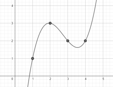
$$P(x) = \frac{2}{3}x^3 - \frac{11}{2}x^2 + \frac{83}{6}x - 8$$

Extending the polynomial simply means evaluation \(P\) at 4 more points, the most natural being 5, 6, 7, and 8. We then get the extended data [7, 21, 48, 92]. Now with the entire data [1, 3, 2, 2, 7, 21, 48, 92], any 4 of those 8 points are enough to reconstruct the same polynomial in order to evaluate it at the missing points to get the original data back.

Note that in practice, we avoid ugly fractions and big exponents making numbers explode to infinity by using modular arithmetic, but the idea is exactly the same.

Data Availability Sampling

Now that we have extended our data with this clever polynomial trick, the following statement becomes true:

If at least half of the extended data is available, then the entire data is available.

Remember that this is the core idea of danksharding: we want to drastically increase the blockchain’s data capacity while preserving every node’s ability to confirm that every byte of data is available for anyone who wants to download it. Now, thanks to erasure coding, the node only has to check that at least half the data is available to make a decision regarding the availability of the entire data.

Okay, that doesn’t sound too clever so far, since we first had to double the data by extending it. But here’s the thing: the node doesn’t actually have to download that much data to check that at least 50% of it is there: the node can simply ask for random samples of the data and perform a couple checks and that should be enough to convince the node with very high probability that all the data is there.

Picture a malicious actor trying to withhold some data from the rest of the network, for example if they’re a mischievous sequencer who did some bad things on an optimistic rollup, and they don’t want anyone to have the data necessary to contest it with a fraud proof. The maximum amount of data they can afford to broadcast to the whole network is just under 50% of the extended data, since anything above that is enough to reconstruct the data and snitch.

Recall that the whole data has been converted into a polynomial, and then extended with as many extra evaluations as there were original points. In our simple example above, we had 4 data points converted into a polynomial of degree 3, then evaluated at 4 more points. Imagine that instead we have 100,000 data points, interpolated into a much bigger polynomial which was then extended with 100,000 more evaluations.

If I’m the malicious actor trying to withhold data, I’m not gonna want to publish more than 99,999 data points from the big list of 200,000 points, since anything more than that is enough to interpolate the same polynomial in order to reconstruct everything. Now your job as a node is to check that at least 50% of the data is available, but without doing the simple thing of downloading everything. How? By turning the whole thing into a probability game, of course!

You pick a number \(i\) between 1 and 200,000 and ask the network for the evaluation of \(P(i)\). The probability that the \(i\) you picked happens to be one of the evaluations I did publish is at most \(\frac{99,999}{200,000} \approx \frac{1}{2}\). You then repeat the process again. The probability that both succeeded is at most \(\frac{1}{4}\). You do it again. And again. After just 30 random checks, the probability that all of them just happened to be one of the minority data points I published is necessarily less than \(\frac{1}{2^{30}} \approx \frac{1}{1,000,000,000}\). As you can see, it doesn’t take very long for me to fail this little game, since there’s no way I could have predicted ahead of time which random numbers you were going to ask for.

There are two things worth noticing:

• 30 is much smaller than 100,000. If each data point holds 32 bytes of information, then the whole exercise only required downloading roughly 1 kilobyte of data to check the availability of ~3 megabytes.
• The number of original data points could have instead been a million, or 10 million, or 5 billion, and 30 random checks would have still given the same one-in-a-billion chance of getting it wrong.

That’s it, that’s danksharding in a nutshell! The person creating the block does the heavy lifting of converting the data into a big polynomial and publishing it, and then every validator does this quick sampling game (alongside normal duties) before attesting to the block. Regular, non-validating nodes also do this sampling game, so that even if 99% of the validator are in on the evil data-withholding scheme, honest nodes will still only follow the fork created by the honest 1% that doesn’t withhold data.

Note that this little sampling game check that data is available for whoever wants to download it: if you personally hold funds on a specific rollup, then it might be worth it to go the extra mile and download the relevant data. But by running a node, you’ll still be participating in enforcing the availability of data for all rollups – even the ones you don’t care about. That’s how the combination of data availability sampling and rollups is basically a cheat code version of execution sharding!

Polynomial Commitment Scheme

The one last polynomial trick missing is what’s known as a polynomial commitment scheme, which is a more complex subject to explain, so I won’t get into too much detail in this section. Basically, it’s what we use to make sure that the random sampling checks aren’t just met with nonsense that doesn’t match the actual polynomial we started with.

I can take a big polynomial of a million degree and “hash” it into a very short commitment \(C\). Then once you have this commitment, I can use it to prove to you that the polynomial evaluates to a specific value \(y\) at a given point \(x\). All you have are four very short values: the commitment \(C\), the point \(x\), the evaluation \(y\) and the proof \(\pi\) and performing a quick check convinces you that \(P(x) = y\) without having to know the million coefficients of the big polynomial.

The polynomial commitment scheme used here is known as KZG, which is actually pretty simple if you’re willing to treat a thing or two as a black box. But for understanding blobspace, it’s worth to take a quick detour to get an understanding about how we can summon this secret value \(s\) that absolutely nobody must know.

Summoning the secret \(s\)

It all has to do with elliptic curve scalar multiplication, which is a pretty complicated branch of math if you’re not already familiar with it. For our purposes however, all you really need to know is that these fancy elliptic curves allow us to craft a function that “encrypts” numbers in a one-way fashion.

Reusing the same notation from earlier, \([x]\) is the encrypted version of \(x\). Aside from being a one-way function (easy to go \(x \rightarrow [x]\), impossible to go \([x] \rightarrow x\)) there are two other important mathematical properties we care about:

1. \(n\cdot[x] = [n\cdot x]\)
2. \([x] + [y] = [x+y]\)

These properties are pretty powerful, because they let us do computations without having to know the values we’re using in the computation. Namely, if you’re given the encrypted powers of \(s\), you can evaluate the encrypted version of \(P(s)\) without ever knowing the actual value of \(s\):

\(P([s]) = c_0[s^0] + c_1[s^1] + c_2[s^2] +\ ... +\ c_n[s^n]\)
\(= [c_0\cdot1] + [c_1\cdot s] + [c_2\cdot s^2]\ +\ ...\ +\ [c_n\cdot s^n]\)
\(= [c_0\cdot1 + c_1\cdot s + c_2\cdot s^2\ +\ ...\ + c_n\cdot s^n]\)
\(= [P(s)]\)

The only problem remaining is that whoever gave you the encrypted powers of \(s\) necessarily had to know the unencrypted value of \(s\). You have to trust that they deleted their copy of \(s\) after they were done, or that their random generator worked as it should, or that their computer wasn’t being spied on, etc. The solution is to have many participants as possible each computing their own secrets, and then mixing all the secrets together sequentially:

• Alice generates a random number \(a\) and publishes \([a]\), \([a^2]\), \([a^3]\), …
• Bob generates a random number \(b\) and – without knowing \(a\) – computes \(b[a] = [ba]\) and publishes \([ba]\), \(b^2[a^2] = [b^2\cdot a^2] = [(ba)^2]\), \(b^3[a^3] = [(ba)^3]\), …
• Charlie generates a random number \(c\) and – still without knowing either \(a\) or \(b\) – computes \(c[ba] = [cba]\) and publishes \([cba]\), \(c^2[(ba)^2] = [(cba)^2]\), \(c^3[(ba)^3] = [(cba)^3]\), …

Now the secret \(s\) is simply \(cba\), and the only way to get the unencrypted secret is if all three of them kept their random number and agree to collude together to multiply them together. Or in other words, as long as just one person participated honestly and threw away their secret, the resulting final secret \(s\) is safe and nobody in the world knows what it is.

Scale this little secret-summoning ceremony to over a hundred thousand participants, and the probability that all of them collude is effectively 0%. Even better if you participated yourself and know you acted honestly, then absolutely all doubts are taken care of. Thankfully, this is what Ethereum’s own ceremony looked like!

By the way, the proper term for this is a KZG trusted setup, you can read more about it from Vitalik’s blog post here

The blob market

Pricing curve

Blobs will be priced in terms of a new resource, creatively named “blob gas”. The pricing mechanism is very similar to EIP-1559: Once EIP-4844 rolls out, there will be a target of 3 blobs per block along with a hard burst limit of 6 blobs per block. Recall that each blob holds about 125 kb of data, which means blocks will contain on average 375 kb of blob data, but in the extreme can contain twice that much. As usual, these numbers are constants that will be increased once full danksharding rolls out, with all the fancy data availability sampling stuff.

Note that there is a slight difference in how the prices of regular gas and blob gas are calculated:

• Regular gas pricing: The price of gas in a block is a simple function of how much gas was used in the previous block compared to the target.
• Blob gas pricing: The price of blob gas is a function of the running tally excess blobs there have been in total.

Basically, each block will have a new header field tracking this tally of excess blobs, updating it according to how many blobs are included in the block compared to the target. So if the current tally is 500 excess blob and the block includes 0 blobs, that’s 3 blobs below the target so the next block’s tally will be 497. Otherwise, if the block includes 5, that’s 2 blobs above the target so the next block’s tally will be 502.

This running tally then becomes the input to a function that outputs how much blobs should be priced for that block. Just like the EIP-1559, this function has an exponential nature: blocks can only contain 6 blobs for so long before the cost blows up to infinity and nobody can afford to pay it, which will drive the count of excess blobs down until there are willing bidders again.

Both mechanisms achieve the same goal of listing a minimum price (which gets burned, of course) but the difference is pretty interesting to me. This is supposed to make the pricing curve more efficient in targeting the average of 3 blobs per block. Here is an ethresear.ch post about it for more explanation about the math.

2D fee market

Another fun aspect of EIP-4844 is the introduction of the two-dimensional fee market, meaning execution and blobs will be priced separately, according to the individual demand for each. The “price of execution” is simply the gas fees we know today, with EIP-1559 and all that good stuff.

In more concrete terms, this means that Layer 1 could be super congested and expensive (picture an NFT drop or a heated memecoin trading frenzy as we’ve seen before) without affecting the price of blobs, which in turn shields Layer 2 users from suffering the congestion of whatever nonsense is happening at Layer 1.

Just like the fancy running tally mechanism described above, this is another thing that makes Ethereum’s fee market vastly more efficient. Nicknamed “Multidimensional EIP-1559”, the introduction of a completely new type of resource is the perfect excuse to start splitting everything up so that available resources are used as efficiently as possible.

Full Danksharding

Alright, so as stated in the section about history, EIP-4844 sets the stage on the execution layer but doesn’t do any of the fancy data sampling tricks on the consensus layer, defaulting to the simplest data availability of “every node downloads every blob”, which is why blobs start out fairly small.

Full Danksharding entails changes behind the scenes, which will not only allow blobs to be much bigger, but also allow blocks to contain more blobs. Rollups who upgraded to support EIP-4844 won’t have to do anything, from their perspective the only thing that changes is that committing data onchain magically became much cheaper!

The main thing worth noting about this upgrade will be the two-dimensional nature of how data blobs are packed into blocks, and how the data is extended. In the section on erasure coding above, I’ve kept it simple and one-dimensional, where the list of data points gets turned into a single polynomial and then evaluated into an equal number of extra points. In the case of danksharding, however, the concept takes place in a 2D grid:

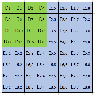
In this simplified example, there are 16 original data points (the green D’s) and 48 extended evaluation points (the blue E’s). Any 4 points in a row are enough to reconstruct the entire row, and likewise for columns. This helps progressively reconstruct the entire square when a reconstructed row gives new information on a column and vice-versa – kind of like a sudoku game, in a way.

Some things we quickly notice from doing this 2D thing is that the total extended data is 4 times bigger than the original data, as opposed to just 2. And the statement we had that “if 50% of the data is available, all the data is available” is updated with a figure of 75%. But the idea of doing random sampling checks works the same, we just have to do a bit more to get the same one-in-a-billion chance of being fooled.

The reason to do it this way is that we can split the responsibility of holding all those polynomials into more manageable rows and columns, and assign them to various validators – this way no node is required to know the entire square. The math also works out in such a way that if validators pick just 2 random rows and columns and do the sampling game exclusively on them to decide whether or not to attest to the whole block, an incomplete block (i.e less than 75% was published) cannot get more than \(\frac{1}{16}\) of attestations, which makes it very unlikely to get included in the main chain.

Additionally, the polynomial commitment scheme used (KZG) has some extra complicated properties that further simplify things in the 2D grid.

What’s left

At this point the theory behind danksharding and data availability sampling is pretty solid. The main things left to solve are mainly from a practical implementation standpoint, especially at a peer-to-peer networking level. Among other things, we want sampling clients and ways to efficiently reconstruct the data is an ongoing topic of research.

Thankfully, by itself EIP-4844 buys us a lot of time to solve these problems and implement all the clever polynomial magic in practice.

Further links

• Execution layer specs for EIP-4844 with all the constants and math formula
• Proto-Danksharding FAQ with a lot of the same information as here but a bit more technical
• Danksharding Workshop - Devcon 6 that walks through the numerous steps
• Earlier Danksharding Workshop
• Data recovery: a toy example, a fun article walking through a simplified example of erasure coding to recover data
• Proto-Danksharding theme song

---